Скачать с ютуб AWGN, WGN, Autocorrelation and PSD Explained using Matlab в хорошем качестве
AWGN, WGN, Autocorrelation and PSD Explained using Matlab
3 года назад
awgn
additive white gaussian noise
white noise
white gaussian noise
autocorrelation
auto correlation
signals and systems
power spectral density
power spectral density example
power spectral density of random process
matlab
matlab tutorial
time series data in matlab
how to plot time series data in matlab
psd
gaussian matlab
gaussian distribution
normal distribution
statistics
standard deviation
variance
awgn channel
Скачать бесплатно и смотреть ютуб-видео без блокировок AWGN, WGN, Autocorrelation and PSD Explained using Matlab в качестве 4к (2к / 1080p)
У нас вы можете посмотреть бесплатно AWGN, WGN, Autocorrelation and PSD Explained using Matlab или скачать в максимальном доступном качестве, которое было загружено на ютуб. Для скачивания выберите вариант из формы ниже:
Загрузить музыку / рингтон AWGN, WGN, Autocorrelation and PSD Explained using Matlab в формате MP3:
Если кнопки скачивания не
загрузились
НАЖМИТЕ ЗДЕСЬ или обновите страницу
Если возникают проблемы со скачиванием, пожалуйста напишите в поддержку по адресу внизу
страницы.
Спасибо за использование сервиса savevideohd.ru
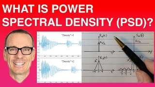
AWGN, WGN, Autocorrelation and PSD Explained using Matlab
Using matlab simulation with code in description of this video, we address what is wgn ,i.e., white Gaussian noise, how to generate awgn ,i.e., additive white Gaussian noise, how to find autocorrelation function of white Gaussian noise and how auto-correlation function relates with the psd , i.e., power spectral density. We look into some of the key concepts which are directly related to the topic of Gaussian distribution such and probability density function of Gaussian random variable, the outcomes within a random process, difficulty of finding psd from the auto correlation function and how does the white Gaussian noise sound. %The matlab code used in the simulation setup presented in the video is given below. clc; clear all; close all fs = 1e4; % Sampling Fre t_span = 10; % max time in sec t = 0:1/fs:t_span-1/fs; % time interval L = size(t,2); % Number of Samples mu=0; % mean value var = .1; % variance aka power in W sigma=sqrt(var); % st. deviation var_dB = 10*log(var); % Power in dBW %Generating the random Process X=sqrt(var)*randn(L,1)+mu; %Stem Time Series Plot of White Gaussian Noise. figure(1); stem(X); title('Stem Time Series Plot of White Gaussian Noise'); xlabel('Samples') ylabel('Sample Values') axis([0 25 -.5 .5]); grid on; grid on; keyboard %Sound of White Gaussian Noise. sound(X) keyboard %Plot the PDF of the Gaussian random variable. figure(2); [f,xi]=ksdensity(X); plot(xi,f,'-o') grid on; title('PDF of White Gaussian Noise'); xlabel('x'); ylabel('PDF f_x(x)'); % Auto-correlation function; The argument 'biased' is used for proper scaling by 1/L %Normalize auto-correlation with sample length for proper scaling [acf,lags] = xcorr(X,'biased'); figure(3) plot(lags,acf); axis([-1000 1000 0 0.02]); grid on; title('Auto-correlation Function of White Noise'); xlabel('Lags (\tau)') ylabel('Auto-correlation = \sigma^2 \delta(\tau)') grid on; keyboard %The PSD part is adopted from %https://www.gaussianwaves.com/2013/11... %A very useful resoruce that is. %Since X is iid, we partition it to approximate PSD figure(4) X1= reshape(X,[1000,100]); w = 1/sqrt(size(X1,1))*fft(X1); %Normalizing by sqrt(size(X1,1)); Pzavg = mean(w.*conj(w)); %Computing the mean power from fft N=size(X1,2); normFreq=[-N/2:N/2-1]/N; Pzavg=fftshift(Pzavg); %Shift zero-frequency component to center of spectrum plot(normFreq,10*log10(Pzavg),'r'); axis([-0.5 0.5 -30 5]); grid on; ylabel('PSD (dB/Hz)'); xlabel('Normalized Frequency'); title('Power Spectral Density (PSD) of White Noise'); keyboard %AWGN on Sawtooth wave figure(5) new_sig = 2*sin(2*t)'; new_sig_noise = new_sig+X; plot(t,new_sig_noise, '-.g') hold on plot(t,new_sig, 'r') legend('Signal with AWGN','Original Signal') xlabel('time') ylabel('Values') grid on;
Comments